13. Analysis
ESPResSo provides two concepts of system analysis:
Direct analysis routines: The
espressomd.analyzemodule provides online-calculation of specialized local and global observables with calculation and data accumulation performed in the core.Observables and correlators: This provides a more flexible concept of in-core analysis, where a certain observable (Available observables), a rule for data accumulation (Accumulators) and/or correlation (Correlations) can be defined.
13.1. Direct analysis routines
The direct analysis commands can be classified into two types:
Instantaneous analysis routines, that only take into account the current configuration of the system:
- Analysis on stored configurations, added by
espressomd.analyze.Analysis.append(): Radial distribution function with
rdf_type='<rdf>'
- Analysis on stored configurations, added by
13.1.1. Energies
espressomd.analyze.Analysis.energy()
Returns the energies of the system. The different energetic contributions to the total energy can also be obtained (kinetic, bonded,non-bonded, Coulomb).
For example,
>>> energy = system.analysis.energy()
>>> print(energy["total"])
>>> print(energy["kinetic"])
>>> print(energy["bonded"])
>>> print(energy["non_bonded"])
13.1.2. Momentum of the System
espressomd.analyze.Analysis.linear_momentum()
This command returns the total linear momentum of the particles and the lattice-Boltzmann (LB) fluid, if one exists. Giving the optional parameters either causes the command to ignore the contribution of LB or of the particles.
13.1.3. Minimal distances between particles
espressomd.analyze.Analysis.min_dist()
Returns the minimal distance between all particles in the system.
When used with type-lists as arguments, then the minimal distance between particles of only those types is determined.
espressomd.analyze.Analysis.dist_to()
Returns the minimal distance of all particles to either a particle (when used with an argument id)
or a position coordinate when used with a vector pos.
For example,
>>> import espressomd
>>> system = espressomd.System(box_l=[100, 100, 100])
>>> for i in range(10):
...     system.part.add(id=i, pos=[1.0, 1.0, i**2], type=0)
>>> system.analysis.dist_to(id=4)
7.0
>>> system.analysis.dist_to(pos=[0, 0, 0])
1.4142135623730951
>>> system.analysis.min_dist()
1.0
13.1.4. Particles in the neighborhood
espressomd.analyze.Analysis.nbhood()
Returns a list of the particle ids of that fall within a given radius of a target position. For example,
idlist = system.analysis.nbhood(pos=system.box_l * 0.5, r_catch=5.0)
13.1.5. Particle distribution
espressomd.analyze.Analysis.distribution()
Returns the distance distribution of particles (probability of finding a particle of a certain type at a specified distance around a particle of another specified type, disregarding the fact that a spherical shell of a larger radius covers a larger volume). The distance is defined as the minimal distance between a particle of one group to any of the other group.
Two arrays are returned corresponding to the normalized distribution and the bins midpoints, for example
>>> system = espressomd.System(box_l=[10, 10, 10])
>>> for i in range(5):
...     system.part.add(id=i, pos=i * system.box_l, type=0)
>>> bins, count = system.analysis.distribution(type_list_a=[0], type_list_b=[0],
...                                            r_min=0.0, r_max=10.0, r_bins=10)
>>>
>>> print(bins)
[ 0.5  1.5  2.5  3.5  4.5  5.5  6.5  7.5  8.5  9.5]
>>> print(count)
[ 1.  0.  0.  0.  0.  0.  0.  0.  0.  0.]
13.1.6. Cylindrical Average
espressomd.analyze.Analysis.cylindrical_average()
Calculates the particle distribution using cylindrical binning.
The volume considered is inside a cylinder defined by the parameters center, axis, length and radius.
The geometrical details of the cylindrical binning is defined using bins_axial and bins_radial which are the number bins in the axial and radial directions (respectively).
See figure Geometry for the cylindrical binning for a visual representation of the binning geometry.
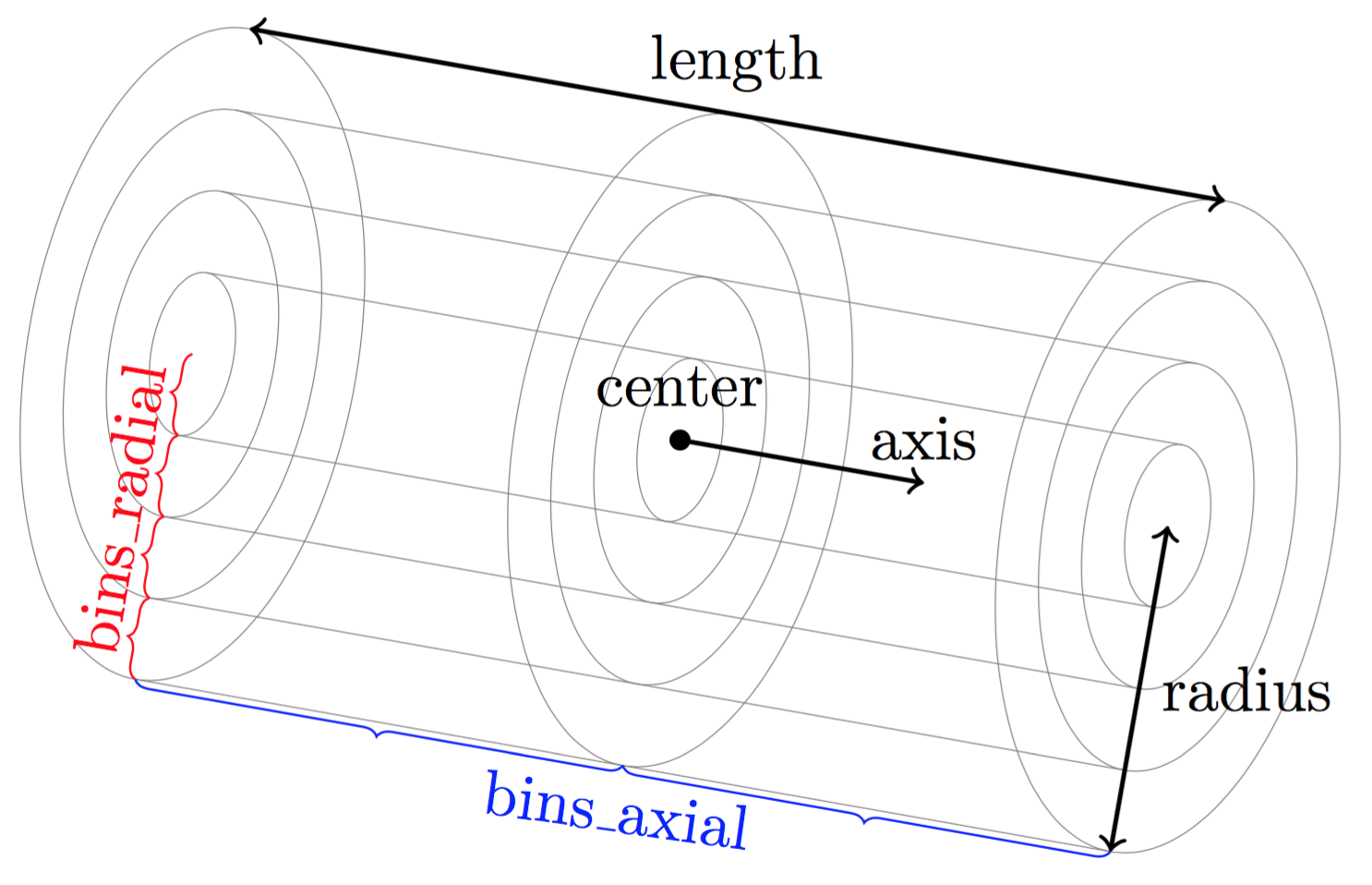
Geometry for the cylindrical binning
The command returns a list of lists. The outer list contains all data combined whereas each inner list contains one line. Each lines stores a different combination of the radial and axial index. The output might look something like this
[ [ 0 0 0.05 -0.25 0.0314159 0 0 0 0 0 0 ]
  [ 0 1 0.05 0.25 0.0314159 31.831 1.41421 1 0 0 0 ]
  ... ]
In this case two different particle types were present. The columns of the respective lines are coded like this
index_radial |
index_axial |
pos_radial |
pos_axial |
binvolume |
density |
v_radial |
v_axial |
density |
v_radial |
v_axial |
|---|---|---|---|---|---|---|---|---|---|---|
0 |
0 |
0.05 |
-0.25 |
0.0314159 |
0 |
0 |
0 |
0 |
0 |
0 |
0 |
1 |
0.05 |
0.25 |
0.0314159 |
31.831 |
1.41421 |
1 |
0 |
0 |
0 |
As one can see the columns density, v_radial and v_axial appear twice.
The order of appearance corresponds to the order of the types in the argument types.
For example if was set to types=[0, 1] then the first triple is associated to type 0 and
the second triple to type 1.
13.1.7. Radial distribution function
espressomd.analyze.Analysis.rdf()
Calculates a radial distribution function for given particle type and binning.
The rdf_type defines if the analysis is performed on the current configuration (rdf_type='rdf')
or on averaged configurations stored with analyze.append() (rdf_type='<rdf>').
For example,
rdf_bins = 100
r_min = 0.0
r_max = system.box_l[0] / 2.0
r, rdf_01 = S.analysis.rdf(rdf_type='<rdf>', type_list_a=[0], type_list_b=[1],
                           r_min=r_min, r_max=r_max, r_bins=rdf_bins)
rdf_fp = open("rdf.dat", 'w')
for i in range(rdf_bins):
    rdf_fp.write("%1.5e %1.5e %1.5e %1.5e\n" % (r[i], rdf_01[i]))
rdf_fp.close()
13.1.8. Structure factor
espressomd.analyze.Analysis.structure_factor()
Calculate the structure factor for given types.
Returns the spherically averaged structure factor \(S(q)\) of
particles specified in sf_types. \(S(q)\) is calculated for all possible
wave vectors \(\frac{2\pi}{L} \leq q \leq \frac{2\pi}{L}\) up to sf_order.
13.1.9. Center of mass
espressomd.analyze.Analysis.center_of_mass()
Returns the center of mass of particles of the given type given by part_type.
13.1.10. Moment of inertia matrix
espressomd.analyze.Analysis.moment_of_inertia_matrix()
Returns the 3x3 moment of inertia matrix for particles of a given type.
13.1.11. Gyration tensor
espressomd.analyze.Analysis.gyration_tensor()
Analyze the gyration tensor of particles of a given type, or of all particles in the system if no type is given. Returns a dictionary containing the squared radius of gyration, three shape descriptors (asphericity, acylindricity, and relative shape anisotropy), eigenvalues of the gyration tensor and their corresponding eigenvectors. The eigenvalues are sorted in descending order.
13.1.12. Pressure
espressomd.analyze.Analysis.pressure()
Computes the instantaneous virial pressure for an isotropic and homogeneous system. It
returns all the contributions to the total pressure as well as the total pressure (see espressomd.analyze.Analysis.pressure()).
The instantaneous pressure is calculated (if there are no electrostatic interactions) by the volume averaged, direction averaged instantaneous virial pressure
where \(f=3\) is the number of translational degrees of freedom of each particle, \(V\) is the volume of the system, \(E_{\text{kinetic}}\) is the kinetic energy, \(F_{ij}\) the force between particles i and j, and \(r_{ij}\) is the distance between them. The kinetic energy divided by the degrees of freedom is
Note that Equation (1) can only be applied to pair potentials and central forces. Description of how contributions from other interactions are calculated is beyond the scope of this manual. Three body potentials are implemented following the procedure in Ref. [TPM09]. A different formula is used to calculate contribution from electrostatic interactions. For electrostatic interactions in P3M, the \(k\)-space contribution is implemented according to [EPB+95]. The implementation of the Coulomb P3M pressure is tested against LAMMPS.
Four-body dihedral potentials are not included. Except of
VIRTUAL_SITES_RELATIVE constraints all other
constraints of any kind are not currently accounted for in the pressure
calculations. The pressure is no longer correct, e.g., when particles
are confined to a plane.
Note: The different contributions which are returned are the summands that arise from force splitting \(\vec{F}_{i,j}={\vec{F}_{i,j}}_\text{bonded}+{\vec{F}_{i,j}}_\text{nonbonded}+...\) in the virial pressure formula. Later when the user calculates the ensemble average via e.g. \(\langle p \rangle \approx 1/N \sum_{i=1}^N p_i\) however the ensemble average with all interactions present is performed. That means the contributions are not easy to interpret! Those are the contributions to the stress/pressure in a system where all interactions are present and therefore in a coupled system.
13.1.13. Stress Tensor
espressomd.analyze.Analysis.stress_tensor()
Computes the volume averaged instantaneous stress tensor of the system with options which are
described by in espressomd.analyze.Analysis.stress_tensor(). It is called a stress tensor but the sign convention follows that of a pressure tensor.
In general do only use it for (on average) homogeneous systems. For inhomogeneous systems you need to use the local stress tensor.
The instantaneous virial stress tensor is calculated by
where the notation is the same as for the pressure. The superscripts \(k\) and \(l\) correspond to the components in the tensors and vectors.
If electrostatic interactions are present then also the coulombic parts of the stress tensor need to be calculated. If P3M is present, then the instantaneous stress tensor is added to the above equation in accordance with [EPB+95] :
where the first summand is the short ranged part and the second summand is the long ranged part.
The short ranged part is given by:
where \(\beta\) is the P3M splitting parameter, \(\vec{n}\) identifies the periodic images, the asterisk denotes that terms with \(\vec{n}=\vec{0}\) and i=j are omitted. The long ranged (k-space) part is given by:
where \(S(\vec{k})\) is the Fourier transformed charge density. Compared to Essmann we do not have the contribution \(p^\text{corr}_{k,l}\) since we want to calculate the pressure that arises from all particles in the system.
Note: The different contributions which are returned are the summands that arise from force splitting \(\vec{F}_{i,j}={\vec{F}_{i,j}}_\text{bonded}+{\vec{F}_{i,j}}_\text{nonbonded}+...\) in the virial stress tensor formula. Later when the user calculates the stress tensor via \(\langle p_{(k,l)}\rangle \approx 1/N \sum_{i=1}^N p_{k,l}\) however the ensemble average with all interactions present is performed. That means the contributions are not easy to interpret! Those are the contributions to the stress/pressure in a system where all interactions are present and therefore in a coupled system.
Note that the angular velocities of the particles are not included in the calculation of the stress tensor.
13.1.14. Chains
All analysis functions in this section require the topology of the chains to be set correctly. The above set of functions is designed to facilitate analysis of molecules. Molecules are expected to be a group of particles comprising a contiguous range of particle IDs. Each molecule is a set of consecutively numbered particles and all molecules are supposed to consist of the same number of particles.
Some functions in this group require that the particles constituting a molecule are connected into linear chains (particle \(n\) is connected to \(n+1\) and so on) while others are applicable to molecules of whatever topology.
13.1.14.1. End-to-end distance
espressomd.analyze.Analysis.calc_re()
Returns the quadratic end-to-end-distance and its root averaged over all chains.
13.1.14.2. Radius of gyration
espressomd.analyze.Analysis.calc_rg()
Returns the radius of gyration averaged over all chains. It is a radius of a sphere, which would have the same moment of inertia as the molecule, defined as
where \(\vec r_i\) are position vectors of individual particles constituting a molecule and \(\vec r_{\mathrm{cm}}\) is the position vector of its center of mass. The sum runs over all \(N\) particles comprising the molecule. For more information see any polymer science book, e.g. [RC03].
13.1.14.3. Hydrodynamic radius
espressomd.analyze.Analysis.calc_rh()
Returns the hydrodynamic radius averaged over all chains. The following formula is used for the computation:
The above-mentioned formula is only valid under certain assumptions. For more information, see Chapter 4 and equation 4.102 in [DE86]. Note that the hydrodynamic radius is sometimes defined in a similar fashion but with a denominator of \(N^2\) instead of \(N(N-1)\) in the prefactor. Both versions are equivalent in the \(N\rightarrow \infty\) limit but give numerically different values for finite polymers.
13.2. Observables and correlators
Analysis in the core is a new concept introduced in since version 3.1. It was motivated by the fact, that sometimes it is desirable that the analysis functions do more than just return a value to the scripting interface. For some observables it is desirable to be sampled every few integration steps. In addition, it should be possible to pass the observable values to other functions which compute history-dependent quantities, such as correlation functions. All this should be done without the need to interrupt the integration by passing the control to the script level and back, which produces a significant overhead when performed too often.
Some observables in the core have their corresponding counterparts in
the espressomd.analyze module. However, only the core-observables can be used
on the fly with the toolbox of the correlator and on the fly analysis of
time series.
Similarly, some special cases of using the correlator have
their redundant counterparts in espressomd.analyze,
but the correlator provides a general and
versatile toolbox which can be used with any implemented
core-observables.
The first step of the core analysis is to create an observable. An observable in the sense of the core analysis can be considered as a rule how to compute a certain set of numbers from a given state of the system or a role how to collect data from other observables. Any observable is represented as a single array of double values. Any more complex shape (tensor, complex number, …) must be compatible to this prerequisite. Every observable however documents the storage order.
The observables can be used in parallel simulations. However, not all observables carry out their calculations in parallel. Instead, the entire particle configuration is collected on the head node, and the calculations are carried out there. This is only performance-relevant if the number of processor cores is large and/or interactions are calculated very frequently.
13.2.1. Creating an observable
The observables are represented as Python classes derived from espressomd.observables.Observable. They are contained in
the espressomd.observables module. An observable is instantiated as
follows
from espressomd.observables import ParticlePositions
part_pos = ParticlePositions(ids=(1, 2, 3, 4, 5))
Here, the keyword argument ids specifies the ids of the particles,
which the observable should take into account.
The current value of an observable can be obtained using its calculate()-method:
print(part_pos.calculate())
13.2.2. Available observables
The following list contains some of the available observables. You can find documentation for
all available observables in espressomd.observables.
Observables working on a given set of particles:
ParticlePositions: Positions of the particlesParticleVelocities: Velocities of the particlesParticleForces: Forces on the particlesParticleBodyVelocities: The particles’ velocities in their respective body-fixed frames (as per their orientation in space stored in their quaternions).ParticleAngularVelocities: The particles’ angular velocities in the space-fixed frameParticleBodyAngularVelocities: As above, but in the particles’ body-fixed frame.
Observables working on a given set of particles and returning reduced quantities:
Current: Total current of the systemDipoleMoment: Total electric dipole moment of the system obtained based on unfolded positionsMagneticDipoleMoment: Total magnetic dipole moment of the system based on theespressomd.particle_data.ParticleHandle.dipproperty.ComPosition: The system’s center of mass based on unfolded coordinatesComVelocity: Velocity of the center of massComForce: Sum of the forces on the particlesParticleDistances: Distances between particles on a polymer chain.BondAngles: Angles between bonds on a polymer chain.BondDihedrals: Dihedral angles between bond triples on a polymer chain.CosPersistenceAngles: Cosine of angles between bonds. Thei-th value in the result vector corresponds to the cosine of the angle between bonds that are separated byibonds. This observable might be useful for measuring the persistence length of a polymer.
Profile observables sampling the spatial profile of various quantities:
Observables sampling the cylindrical profile of various quantities:
System-wide observables
StressTensor: Total stress tensor (see Stress Tensor)
13.2.3. Correlations
Time correlation functions are ubiquitous in statistical mechanics and molecular simulations when dynamical properties of many-body systems are concerned. A prominent example is the velocity autocorrelation function, \(\left< \mathbf{v}(t) \cdot \mathbf{v}(t+\tau) \right>\) which is used in the Green-Kubo relations. In general, time correlation functions are of the form
where \(t\) is time, \(\tau\) is the lag time (time difference) between the measurements of (vector) observables \(A\) and \(B\), and \(\otimes\) is an operator which produces the vector quantity \(C\) from \(A\) and \(B\). The ensemble average \(\left< \cdot \right>\) is taken over all time origins \(t\). Correlation functions describing dynamics of large and complex molecules such as polymers span many orders of magnitude, ranging from MD time step up to the total simulation time.
A correlator takes one or two observables, obtains values from them during the simulation and finally uses a fast correlation algorithm which enables efficient computation of correlation functions spanning many orders of magnitude in the lag time.
The implementation for computing averages and error estimates of a time series of observables relies on estimates of autocorrelation functions and the respective autocorrelation times. The correlator provides the same functionality as a by-product of computing the correlation function.
An example of the usage of observables and correlations is provided in
the script samples/observables_correlators.py.
13.2.3.1. Creating a correlation
Each correlator is represented by an instance of the espressomd.accumulators.Correlator. Please see its documentation for an explanation of the arguments that have to be passed to the constructor.
Correlators can be registered for automatic updating during the
integration by adding them to espressomd.system.System.auto_update_accumulators.
system.auto_update_accumulators.add(corr)
Alternatively, an update can triggered by calling the update() method of the correlator instance. In that case, one has to make sure to call the update in the correct time intervals.
The current on-the-fly correlation result can of a correlator can be obtained using its result() method.
The final result (including the latest data in the buffers) is obtained using the finalize() method. After this, no further update of the correlator is possible.
13.2.3.2. Example: Calculating a particle’s diffusion coefficient
For setting up an observable and correlator to obtain the mean square displacement of particle 0, use:
pos_obs = ParticlePositions(ids=(0,))
c_pos = Correlator(obs1=pos_obs, tau_lin=16, tau_max=100., delta_N=10,
                   corr_operation="square_distance_componentwise", compress1="discard1")
To obtain the velocity auto-correlation function of particle 0, use:
obs = ParticleVelocities(ids=(0,))
c_vel = Correlator(obs1=vel_obs, tau_lin=16, tau_max=20., delta_N=1,
                   corr_operation="scalar_product", compress1="discard1")
The full example can be found in samples/diffusion_coefficient.py.
13.2.4. Details of the multiple tau correlation algorithm
Here we briefly describe the multiple tau correlator which is implemented in ESPResSo. For a more detailed description and discussion of its behavior with respect to statistical and systematic errors, please read the cited literature. This type of correlator has been in use for years in the analysis of dynamic light scattering [SchatzelDS88]. About a decade later it found its way to the Fluorescence Correlation Spectroscopy (FCS) [MF01]. The book of Frenkel and Smit [FS02] describes its application for the special case of the velocity autocorrelation function.
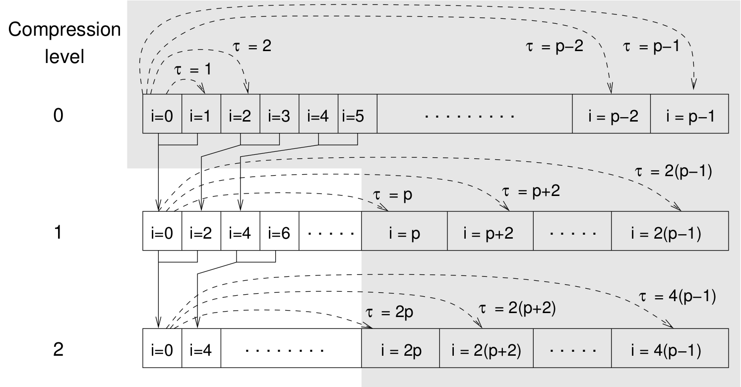
Schematic representation of buffers in the correlator.
Let us consider a set of \(N\) observable values as schematically shown in the figure above, where a value of index \(i\) was measured at times \(i\delta t\). We are interested in computing the correlation function for a range of lag times \(\tau = (i-j)\delta t\) between the measurements \(i\) and \(j\). To simplify the notation, we drop \(\delta t\) when referring to observables and lag times.
The trivial implementation takes all possible pairs of values
corresponding to lag times
\(\tau \in [{\tau_{\mathrm{min}}}:{\tau_{\mathrm{max}}}]\). Without
loss of generality, we consider
\({\tau_{\mathrm{min}}}=0\). The computational effort for such an
algorithm scales as
\({\cal O} \bigl({\tau_{\mathrm{max}}}^2\bigr)\). As a rule of
thumb, this is feasible if \({\tau_{\mathrm{max}}}< 10^3\). The
multiple tau correlator provides a solution to compute the correlation
functions for arbitrary range of the lag times by coarse-graining the
high \(\tau\) values. It applies the naive algorithm to a relatively
small range of lag times \(\tau \in [0:p-1]\)
(\(p\) corresponds to parameter tau_lin).
This we refer to as compression level 0.
To compute the correlations for lag times
\(\tau \in [p:2(p-1)]\), the original data are first coarse-grained,
so that \(m\) values of the original data are compressed to produce
a single data point in the higher compression level. Thus the lag time
between the neighboring values in the higher compression level
increases by a factor of \(m\), while the number of stored values
decreases by the same factor and the number of correlation operations at
this level reduces by a factor of \(m^2\). Correlations for lag
times \(\tau \in [2p:4(p-1)]\) are computed at compression level 2,
which is created in an analogous manner from level 1. This can continue
hierarchically up to an arbitrary level for which enough data is
available. Due to the hierarchical reduction of the data, the algorithm
scales as
\({\cal O} \bigl( p^2 \log({\tau_{\mathrm{max}}}) \bigr)\). Thus an
additional order of magnitude in \({\tau_{\mathrm{max}}}\) costs
just a constant extra effort.
The speedup is gained at the expense of statistical accuracy. The loss of accuracy occurs at the compression step. In principle one can use any value of \(m\) and \(p\) to tune the algorithm performance. However, it turns out that using a high \(m\) dilutes the data at high \(\tau\). Therefore \(m=2\) is hard-coded in the correlator and cannot be modified by user. The value of \(p\) remains an adjustable parameter which can be modified by user by setting when defining a correlation. In general, one should choose \(p \gg m\) to avoid loss of statistical accuracy. Choosing \(p=16\) seems to be safe but it may depend on the properties of the analyzed correlation functions. A detailed analysis has been performed in Ref. [RSVL10].
The choice of the compression function also influences the statistical accuracy and can even lead to systematic errors. The default compression function is which discards the second for the compressed values and pushes the first one to the higher level. This is robust and can be applied universally to any combination of observables and correlation operation. On the other hand, it reduces the statistical accuracy as the compression level increases. In many cases, the compression operation can be applied, which averages the two neighboring values and the average then enters the higher level, preserving almost the full statistical accuracy of the original data. In general, if averaging can be safely used or not, depends on the properties of the difference
For example in the case of velocity autocorrelation function, the above-mentioned difference has a small value and a random sign, different contributions cancel each other. On the other hand, in the of the case of mean square displacement the difference is always positive, resulting in a non-negligible systematic error. A more general discussion is presented in Ref. [RSVL10].
13.3. Accumulators
13.3.1. Time series
In order to take snapshots of an observable,
espressomd.accumulators.TimeSeries can be used:
import espressomd
import espressomd.observables
import espressomd.accumulators

system = espressomd.System(box_l=[10.0, 10.0, 10.0])
system.cell_system.skin = 0.4
system.time_step = 0.01
system.part.add(id=0, pos=[5.0, 5.0, 5.0], v=[0, 2, 0])
position_observable = espressomd.observables.ParticlePositions(ids=(0,))
accumulator = espressomd.accumulators.TimeSeries(
    obs=position_observable, delta_N=2)
system.auto_update_accumulators.add(accumulator)
system.integrator.run(10)
print(accumulator.time_series())
In the example above the automatic update of the accumulator is used. However,
it’s also possible to manually update the accumulator by calling
espressomd.accumulators.TimeSeries.update().
13.3.2. Mean-variance calculator
In order to calculate the running mean and variance of an observable,
espressomd.accumulators.MeanVarianceCalculator can be used:
import espressomd
import espressomd.observables
import espressomd.accumulators

system = espressomd.System(box_l=[10.0, 10.0, 10.0])
system.cell_system.skin = 0.4
system.time_step = 0.01
system.part.add(id=0, pos=[5.0, 5.0, 5.0], v=[0, 2, 0])
position_observable = espressomd.observables.ParticlePositions(ids=(0,))
accumulator = espressomd.accumulators.MeanVarianceCalculator(
    obs=position_observable, delta_N=2)
system.auto_update_accumulators.add(accumulator)
system.integrator.run(10)
print(accumulator.get_mean())
print(accumulator.get_variance())
In the example above the automatic update of the accumulator is used. However,
it’s also possible to manually update the accumulator by calling
espressomd.accumulators.MeanVarianceCalculator.update().
13.4. Cluster analysis
ESPResSo provides support for online cluster analysis. Here, a cluster is a group of particles, such that you can get from any particle to any second particle by at least one path of neighboring particles. I.e., if particle B is a neighbor of particle A, particle C is a neighbor of A and particle D is a neighbor of particle B, all four particles are part of the same cluster. The cluster analysis is available in parallel simulations, but the analysis is carried out on the head node, only.
Whether or not two particles are neighbors is defined by a pair criterion. The available criteria can be found in espressomd.pair_criteria.
For example, a distance criterion which will consider particles as neighbors if they are closer than 0.11 is created as follows:
from espressomd.pair_criteria import DistanceCriterion
dc = DistanceCriterion(cut_off=0.11)
To obtain the cluster structure of a system, an instance of espressomd.cluster_analysis.ClusterStructure has to be created.
To to create a cluster structure with above criterion:
from espressomd.cluster_analysis import ClusterStructure
cs = ClusterStructure(distance_criterion=dc)
In most cases, the cluster analysis is carried out by calling the espressomd.cluster_analysis.ClusterStructure.run_for_all_pairs method. When the pair criterion is purely based on bonds, espressomd.cluster_analysis.ClusterStructure.run_for_bonded_particles can be used.
The results can be accessed via ClusterStructure.clusters, which is an instance of
espressomd.cluster_analysis.Clusters.
Individual clusters are represented by instances of
espressomd.cluster_analysis.Cluster, which provides access to the particles contained in a cluster as well as per-cluster analysis routines such as radius of gyration, center of mass and longest distance.
Note that the cluster objects do not contain copies of the particles, but refer to the particles in the simulation. Hence, the objects become outdated if the simulation system changes. On the other hand, it is possible to directly manipulate the particles contained in a cluster.