8. Bonded interactions
Bonded interactions are configured by the
espressomd.interactions.BondedInteractions class, which is
a member of espressomd.system.System. Generally, one may use
the following syntax to activate and assign a bonded interaction:
system.bonded_inter.add(bond)
p1.add_bond((bond, p2, ...))
In general, one instantiates an interaction object bond and subsequently passes it
to espressomd.interactions.BondedInteractions.add(). This will enable the
bonded interaction and allows the user to assign bonds between particles p1
and p2.
Bonded interactions are identified by either their bondid or their appropriate object.
Defining a bond between two particles always involves three steps:
defining the interaction, adding it to the system and applying it to the particles.
To illustrate this, assume that two particles p1 and p2 already exist.
One could for example create a FENE bond (more information about the FENE bond
is provided in subsection FENE bond) between them using:
fene = FeneBond(k=1, d_r_max=1)
system.bonded_inter.add(fene)
p1.add_bond((fene, p2))
Note that the fene object specifies the type of bond and its parameters,
while the information of the bond between p1 and its bonded partners
is stored on p1. This means that to remove a bond, one has to remember
on which particle the bond was added. You can find more
information regarding particle properties in Setting up particles.
To delete the FENE bond between particles p1 and p2:
p1.delete_bond((fene, p2))
Note that alternatively to particle handles, the particle’s ids can be used to setup bonded interactions. For example, to create a bond between the particles with the ids 12 and 43:
system.part.by_id(12).add_bond((fene, 43))
8.1. Distance-dependent bonds
8.1.1. FENE bond
A FENE (finite extension nonlinear elastic) bond can be instantiated via
espressomd.interactions.FeneBond:
import espressomd.interactions
fene = espressomd.interactions.FeneBond(k=<float>, d_r_max=<float>, r_0=<float>)
This command creates a bond type identifier with a FENE interaction. The FENE potential
models a rubber-band-like, symmetric interaction between two particles with magnitude \(K\), maximal stretching length \(\Delta r_\mathrm{max}\) and equilibrium bond length \(r_0\). The bond potential diverges at a particle distance \(r=r_0-\Delta r_\mathrm{max}\) and \(r=r_0+\Delta r_\mathrm{max}\).
8.1.2. Harmonic bond
A harmonic bond can be instantiated via
espressomd.interactions.HarmonicBond:
import espressomd.interactions
hb = espressomd.interactions.HarmonicBond(k=<float>, r_0=<float>, r_cut=<float>)
This creates a bond type identifier with a classical harmonic potential. It is a symmetric interaction between two particles. It is given by
with \(r_0\) the equilibrium length and \(k\) the magnitude. The third, optional parameter defines a cutoff radius. Whenever a harmonic bond gets longer than \(r_\mathrm{cut}\), the bond will be reported as broken, and a background error will be raised.
8.1.3. Quartic bond
Note
The parameter math:r corresponds to math:r_0 here.
A quartic bond can be instantiated via
espressomd.interactions.QuarticBond:
import espressomd.interactions
qb = espressomd.interactions.QuarticBond(k0=<float>, k1=<float>, r=<float>, r_cut=<float>)
The potential is minimal at particle distance \(r=r_0\). It is given by
The fourth parameter defines a cutoff radius. Whenever a
quartic bond gets longer than r_cut, the bond will be reported as broken, and
a background error will be raised.
8.1.4. Bonded Coulomb
Note
Requires ELECTROSTATICS feature.
A pairwise Coulomb interaction can be instantiated via
espressomd.interactions.BondedCoulomb:
import espressomd.interactions
bonded_coulomb = espressomd.interactions.BondedCoulomb(prefactor=1.0)
system.bonded_inter.add(bonded_coulomb)
p1.add_bond((bonded_coulomb, p2))
This creates a bond with a Coulomb pair potential between particles p1 and p2.
It is given by
where \(q_1\) and \(q_2\) are the charges of the bound particles and \(\alpha\) is the Coulomb prefactor. This interaction has no cutoff and acts independently of other Coulomb interactions.
8.1.5. Subtract P3M short-range bond
Note
Requires the P3M feature.
This bond can be instantiated via
espressomd.interactions.BondedCoulombSRBond:
import espressomd.interactions
subtr_p3m_sr = espressomd.interactions.BondedCoulombSRBond(q1q2=<float>)
The parameter q1q2 sets the charge factor of the short-range P3M interaction.
It can differ from the actual particle charges. This specialized bond can be
used to cancel or add only the short-range electrostatic part
of the P3M solver. A use case is described in Particle polarizability with thermalized cold Drude oscillators.
8.1.6. Rigid bonds
Note
Requires BOND_CONSTRAINT feature.
A rigid bond can be instantiated via
espressomd.interactions.RigidBond:
import espressomd.interactions
rig = espressomd.interactions.RigidBond(r=<float>, ptol=<float>, vtol=<float>)
To simulate rigid bonds, ESPResSo uses the Rattle Shake algorithm which satisfies
internal constraints for molecular models with internal constraints,
using Lagrange multipliers.[Andersen, 1983] The constrained bond distance
is named r, the positional tolerance is named ptol and the velocity tolerance
is named vtol.
8.1.7. Thermalized distance bond
A thermalized bond can be instantiated via
espressomd.interactions.ThermalizedBond:
import espressomd.interactions
thermalized_bond = espressomd.interactions.ThermalizedBond(
    temp_com=<float>, gamma_com=<float>,
    temp_distance=<float>, gamma_distance=<float>,
    r_cut=<float>)
system.bonded_inter.add(thermalized_bond)
system.thermostat.set_thermalized_bond(seed=<int>)
This bond can be used to apply Langevin thermalization on the centre of mass and the distance of a particle pair. Each thermostat can have its own temperature and friction coefficient.
The bond is closely related to simulating Particle polarizability with thermalized cold Drude oscillators.
8.1.8. Tabulated distance
A tabulated bond length can be instantiated via
espressomd.interactions.TabulatedDistance:
import espressomd.interactions
tab_dist = espressomd.interactions.TabulatedDistance(
    min=<min>, max=<max>, energy=<energy>, force=<force>)
system.bonded_inter.add(tab_dist)
p1.add_bond((tab_dist, p2))
This creates a bond type identifier with a tabulated potential. The force acts in the direction of the connecting vector between the particles. The bond breaks above the tabulated range, but for distances smaller than the tabulated range, a linear extrapolation based on the first two tabulated force values is used. For details of the interpolation, see Tabulated interaction.
8.1.9. Virtual bonds
A virtual bond can be instantiated via
espressomd.interactions.Virtual:
import espressomd.interactions
vb = espressomd.interactions.Virtual()
This creates a virtual bond type identifier for a pair bond without associated potential or force. It can be used to specify topologies and for some analysis that rely on bonds, or for bonds that should be displayed in the visualizer.
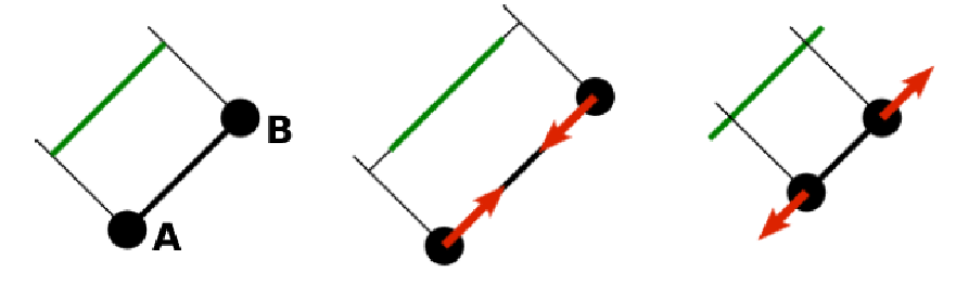
8.2. Bond-angle interactions
Bond-angle interactions involve three particles forming the angle \(\phi\), as shown in the schematic below.

This allows for a bond type having an angle-dependent potential. This potential is defined between three particles and depends on the angle \(\phi\) between the vectors from the central particle to the two other particles.
Similar to other bonded interactions, these are defined for every particle triplet and must be added to a particle (see property bonds), in this case the central one.
For example, for the schematic with particles p0, p1 (central particle) and p2 the bond was defined using
p1.add_bond((bond_angle, p0, p2))
The parameter bond_angle is an instance of one of four possible bond-angle
classes, described below.
8.2.1. Harmonic angle potential
espressomd.interactions.AngleHarmonic
Equation:
\(K\) is the bending constant and \(\phi_0\) is the equilibrium bond angle in radians ranging from 0 to \(\pi\).
Example:
import espressomd.interactions
angle_harmonic = espressomd.interactions.AngleHarmonic(bend=1.0, phi0=2 * np.pi / 3)
system.bonded_inter.add(angle_harmonic)
p1.add_bond((angle_harmonic, p0, p2))
8.2.2. Cosine angle potential
espressomd.interactions.AngleCosine
Equation:
\(K\) is the bending constant and \(\phi_0\) is the equilibrium bond angle in radians ranging from 0 to \(\pi\).
Around \(\phi_0\), this potential is close to a harmonic one (both are \(1/2(\phi-\phi_0)^2\) in leading order), but it is periodic and smooth for all angles \(\phi\).
Example:
import espressomd.interactions
angle_cosine = espressomd.interactions.AngleCosine(bend=1.0, phi0=2 * np.pi / 3)
system.bonded_inter.add(angle_cosine)
p1.add_bond((angle_cosine, p0, p2))
8.2.3. Harmonic cosine potential
espressomd.interactions.AngleCossquare
Equation:
\(K\) is the bending constant and \(\phi_0\) is the equilibrium bond angle in radians ranging from 0 to \(\pi\).
This form is used for example in the GROMOS96 force field. The potential is \(1/8(\phi-\phi_0)^4\) around \(\phi_0\), and therefore much flatter than the two aforementioned potentials.
Example:
import espressomd.interactions
angle_cossquare = espressomd.interactions.AngleCossquare(bend=1.0, phi0=2 * np.pi / 3)
system.bonded_inter.add(angle_cossquare)
p1.add_bond((angle_cossquare, p0, p2))
8.2.4. Tabulated angle potential
A tabulated bond angle can be instantiated via
espressomd.interactions.TabulatedAngle:
import espressomd.interactions
theta = np.linspace(0, np.pi, num=91, endpoint=True)
angle_tab =  espressomd.interactions.TabulatedAngle(
    energy=10 * (theta - 2 * np.pi / 3)**2,
    force=10 * (theta - 2 * np.pi / 3) / 2)
system.bonded_inter.add(angle_tab)
p1.add_bond((angle_tab, p0, p2))
The energy and force tables must be sampled from \(0\) to \(\pi\), where \(\pi\) corresponds to a flat angle. The forces are scaled with the inverse length of the connecting vectors. The force on the extremities acts perpendicular to the connecting vector between the corresponding particle and the center particle, in the plane defined by the three particles. The force on the center particle balances the other two forces. For details of the interpolation, see Tabulated interaction.
8.3. Dihedral interactions
8.3.1. Dihedral potential with phase shift
Dihedral interactions are available through the espressomd.interactions.Dihedral class:
import espressomd.interactions
dihedral = espressomd.interactions.Dihedral(bend=<K>, mult=<n>, phase=<phi_0>)
system.bonded_inter.add(dihedral)
p2.add_bond((dihedral, p1, p3, p4))
This creates a bond type identifier with a dihedral potential, a four-body-potential. In the following, let the particle for which the bond is created be particle \(p_2\), and the other bond partners \(p_1\), \(p_3\), \(p_4\), in this order. Then, the dihedral potential is given by
where \(n\) is the multiplicity of the potential (number of minima) and can take any integer value (typically from 1 to 6), \(\phi_0\) is a phase parameter and \(K\) is the bending constant of the potential. \(\phi\) is the dihedral angle between the particles defined by the particle quadruple \(p_1\), \(p_2\), \(p_3\) and \(p_4\), the angle between the planes defined by the particle triples \(p_1\), \(p_2\) and \(p_3\) and \(p_2\), \(p_3\) and \(p_4\):
Together with appropriate Lennard-Jones interactions, this potential can mimic a large number of atomic torsion potentials.
Note that there is a singularity in the forces, but not in the energy, when \(\phi = 0\) and \(\phi = \pi\).
8.3.2. Tabulated dihedral potential
A tabulated dihedral interaction can be instantiated via
espressomd.interactions.TabulatedDihedral:
import espressomd.interactions
dihedral_tab = espressomd.interactions.TabulatedDihedral(energy=<energy>, force=<force>)
system.bonded_inter.add(dihedral_tab)
p2.add_bond((dihedral_tab, p1, p3, p4))
The energy and force tables must be sampled from \(0\) to \(2\pi\). For details of the interpolation, see Tabulated interaction.
Note that there is a singularity in the forces, but not in the energy, when \(\phi = 0\) and \(\phi = \pi\).
8.4. Immersed Boundary Method interactions
Elastic forces for the Immersed Boundary Method (IBM). With the IBM, soft particles are modelled as a triangulated surface. Each vertex has an associated particle, and neighboring particles have bonded interactions. When the surface is deformed by external forces, elastic forces restore the original geometry [Krüger, 2012].
8.4.1. IBM local forces
8.4.1.1. Shear
espressomd.interactions.IBM_Triel
Compute elastic shear forces. To setup an interaction, use:
tri1 = IBM_Triel(ind1=0, ind2=1, ind3=2, elasticLaw="Skalak", k1=0.1, k2=0, maxDist=2.4)
where ind1, ind2 and ind3 represent the indices of the three
marker points making up the triangle. The parameter maxDist specifies
the maximum stretch above which the bond is considered broken. The parameter
elasticLaw can be either "NeoHookean" or "Skalak".
The parameters k1 and k2 are the elastic moduli.
8.4.1.2. Bending
espressomd.interactions.IBM_Tribend
Compute out-of-plane bending forces. To setup an interaction, use:
tribend = IBM_Tribend(ind1=0, ind2=1, ind3=2, ind4=3, kb=1, refShape="Initial")
where ind1, ind2, ind3 and ind4 are four marker points
corresponding to two neighboring triangles. The indices ind1 and ind3
contain the shared edge. Note that the marker points within a triangle must
be labelled such that the normal vector
\(\vec{n} = (\vec{r}_\text{ind2} - \vec{r}_\text{ind1}) \times (\vec{r}_\text{ind3} - \vec{r}_\text{ind1})\)
points outward of the elastic object. The reference (zero energy) shape
can be either "Flat" or the initial curvature "Initial".
The bending modulus is kb.
8.4.2. IBM global forces
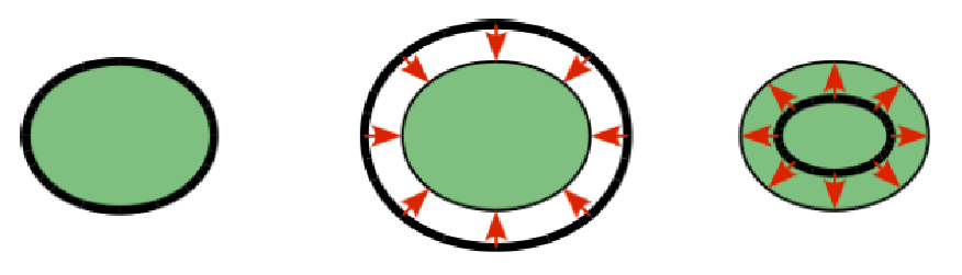
8.4.2.1. Volume conservation
espressomd.interactions.IBM_VolCons
Compute the volume-conservation force. Without this correction, the volume of the soft object tends to shrink over time due to numerical inaccuracies. Therefore, this implements an artificial force intended to keep the volume constant. If volume conservation is to be used for a given soft particle, the interaction must be added to every marker point belonging to that object:
volCons = IBM_VolCons(softID=1, kappaV=kV)
where softID identifies the soft particle and kappaV is a volumetric
spring constant. Note that this volCons bond does not have a bond partner.
It is added to a particle as follows:
system.part.by_id(0).add_bond((volCons,))
The comma is needed to create a tuple containing a single item.
8.5. Object-in-fluid interactions
Please cite [Cimrák et al., 2014] when using the interactions in this section in order to simulate extended objects embedded in a LB fluid. For more details please consult the dedicated OIF documentation available at http://cell-in-fluid.fri.uniza.sk/en/content/oif-espresso.
The following interactions are implemented in order to mimic the mechanics of elastic or rigid objects immersed in the LB fluid flow. Their mathematical formulations were inspired by [Dupin et al., 2007]. Details on how the bonds can be used for modeling objects are described in section Object-in-fluid.
8.5.1. OIF local forces
OIF local forces are available through the espressomd.interactions.OifLocalForces class.
This type of interaction is available for closed 3D immersed objects flowing in the LB flow.
This interaction comprises three different concepts. The local elasticity of biological membranes can be captured by three different elastic moduli. Stretching of the membrane, bending of the membrane and local preservation of the surface area. Parameters \({L^0_{AB}},\ {k_s},\ {k_{s,\mathrm{lin}}}\) define the stretching, parameters \(\phi,\ k_b\) define the bending, and \(A_1,\ A_2,\ k_{al}\) define the preservation of local area. The stretching force is applied first, followed by the bending force and finally the local area force. They can be used all together, or, by setting any of \(k_s, k_{s,\mathrm{lin}}, k_b, k_{al}\) to zero, the corresponding modulus can be turned off.
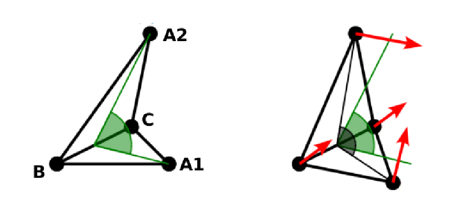
OIF local forces are asymmetric. After creating the interaction
local_inter = OifLocalForces(r0=1.0, ks=0.5, kslin=0.0, phi0=1.7, kb=0.6,
                             A01=0.2, A02=0.3, kal=1.1, kvisc=0.7)
it is important how the bond is created. Particles need to be mentioned in the correct order. Command
p1.add_bond((local_inter, p0.part_id, p2.part_id, p3.part_id))
creates a bond related to the triangles 012 and 123. The particle 0 corresponds to point A1, particle 1 to C, particle 2 to B and particle 3 to A2. There are two rules that need to be fulfilled:
there has to be an edge between particles 1 and 2
orientation of the triangle 012, that is the normal vector defined as a vector product \(01 \times 02\) must point to the inside of the immersed object.
Then the stretching force is applied to particles 1 and 2, with the relaxed length being 1.0. The bending force is applied to preserve the angle between triangles 012 and 123 with relaxed angle 1.7 and finally, local area force is applied to both triangles 012 and 123 with relaxed area of triangle 012 being 0.2 and relaxed area of triangle 123 being 0.3.
8.5.1.1. Stretching
For each edge of the mesh, \(L_{AB}\) is the current distance between point \(A\) and point \(B\). \(L^0_{AB}\) is the distance between these points in the relaxed state, that is if the current edge has this length exactly, then no forces are added. \(\Delta L_{AB}\) is the deviation from the relaxed state, that is \(\Delta L_{AB} = L_{AB} - L_{AB}^0\). The stretching force between \(A\) and \(B\) is calculated using
Here, \(n_{AB}\) is the unit vector pointing from \(A\) to \(B\), \(k_s\) is the constant for nonlinear stretching, \(k_{s,\mathrm{lin}}\) is the constant for linear stretching, \(\lambda_{AB} = L_{AB}/L_{AB}^0\), and \(\kappa\) is a nonlinear function that resembles neo-Hookean behavior
Typically, one wants either nonlinear or linear behavior and therefore one of \(k_s, k_{s,\mathrm{lin}}\) is zero. Nonetheless the interaction will work if both constants are non-zero.
8.5.1.2. Bending
The tendency of an elastic object to maintain the resting shape is achieved by prescribing the preferred angles between neighboring triangles of the mesh.
Denote the angle between two triangles in the resting shape by \(\theta^0\). For closed immersed objects, one always has to set the inner angle. The deviation of this angle \(\Delta \theta = \theta - \theta^0\) defines two bending forces for two triangles \(A_1BC\) and \(A_2BC\)
Here, \(n_{A_iBC}\) is the unit normal vector to the triangle \(A_iBC\). The force \(F_{bi}(A_iBC)\) is assigned to the vertex not belonging to the common edge. The opposite force divided by two is assigned to the two vertices lying on the common edge. This procedure is done twice, for \(i=1\) and for \(i=2\).
Notice that concave objects can be created with \(\theta^0 > \pi\).
8.5.1.3. Local area conservation
This interaction conserves the area of the triangles in the triangulation. The area constraint assigns the following shrinking/expanding force to vertex \(A\):
where \(\Delta S_\triangle\) is the difference between current \(S_\triangle\) and area \(S^0\) of the triangle in relaxed state, \(T\) is the centroid of the triangle, and \(t_a, t_b, t_c\) are the lengths of segments \(AT, BT, CT\), respectively. Similarly the analogue forces are assigned to \(B\) and \(C\).

8.5.2. OIF global forces
OIF global forces are available through the
espressomd.interactions.OifGlobalForces class.
This type of interaction is available solely for closed 3D immersed objects.
It comprises two concepts: preservation of global surface and of volume of the object. The parameters \(S^0, k_{ag}\) define preservation of the surface while parameters \(V^0, k_{v}\) define volume preservation. They can be used together, or, by setting either \(k_{ag}\) or \(k_{v}\) to zero, the corresponding modulus can be turned off.
These interactions are symmetric. After the definition of the interaction by
global_force_interaction = OifGlobalForces(A0_g=65.3, ka_g=3.0, V0=57.0, kv=2.0)
the order of vertices is crucial. By the following command the bonds are defined
p0.add_bond((global_force_interaction, p1.part_id, p2.part_id))
Triangle 012 must have correct orientation, that is the normal vector defined by a vector product \(01\times02\) must point to the inside of the immersed object.
8.5.2.1. Global area conservation
The global area conservation force is defined as
where \(S^c\) denotes the current surface of the immersed object, \(S^c_0\) the surface in the relaxed state, \(S_{ABC}\) is the surface of the triangle, \(T\) is the centroid of the triangle, and \(t_a, t_b, t_c\) are the lengths of segments \(AT, BT, CT\), respectively.
8.5.2.2. Volume conservation
The deviation of the objects volume \(V\) is computed from the volume in the resting shape \(\Delta V = V - V^0\). For each triangle, the following force is computed:
where \(S_{ABC}\) is the area of triangle \(ABC\), \(n_{ABC}\) is the normal unit vector of the plane spanned by \(ABC\), and \(k_v\) is the volume constraint coefficient. The volume of one immersed object is computed from
where the sum is computed over all triangles of the mesh and \(h_{ABC}\) is the normal vector from the centroid of triangle \(ABC\) to any plane which does not cross the cell. The force \(F_v(ABC)\) is equally distributed to all three vertices \(A, B, C.\)