18. Advanced methods
This page documents advanced features of ESPResSo. Be sure to read the relevant literature before using them.
18.1. Creating bonds when particles collide
Please cite [Arnold et al., 2013] when using dynamic binding.
With the help of this feature, bonds between particles can be created automatically during the simulation, every time two particles collide. This is useful for simulations of chemical reactions and irreversible adhesion processes. Both, sliding and non-sliding contacts can be created.
The collision detection is controlled via the system
collision_detection attribute,
which is an instance of the class
CollisionDetection.
Several modes are available for different types of binding.
"bind_centers": adds a pair-bond between two particles at their first collision. By making the bonded interaction stiff enough, the particles can be held together after the collision. Note that the particles can still slide on each others’ surface, as the pair bond is not directional. This mode is set up as follows:import espressomd import espressomd.interactions system = espressomd.System(box_l=[1, 1, 1]) bond_centers = espressomd.interactions.HarmonicBond(k=1000, r_0=1.5) system.bonded_inter.add(bond_centers) system.collision_detection.set_params(mode="bind_centers", distance=1.5, bond_centers=bond_centers)
The parameters are as follows:
distanceis the distance between two particles at which the binding is triggered. This cutoff distance,1.5in the example above, is typically chosen slightly larger than the particle diameter. It is also a good choice for the equilibrium length of the bond.bond_centersis the bonded interaction to be created between the particles (an instance ofHarmonicBondin the example above). No guarantees are made regarding which of the two colliding particles gets the bond. Once there is a bond of this type on any of the colliding particles, no further binding occurs for this pair of particles.
"bind_at_point_of_collision": this mode prevents sliding of the colliding particles at the contact. This is achieved by creating two virtual sites at the point of collision. They are rigidly connected to each of the colliding particles. A bond is then created between the virtual sites, or an angular bond between the two colliding particles and the virtual particles. In the latter case, the virtual particles are the centers of the angle potentials (particle 2 in the description of the angle potential, see Bond-angle interactions). Due to the rigid connection between each of the particles in the collision and its respective virtual site, a sliding at the contact point is no longer possible. See the documentation on Rigid arrangements of particles for details. In addition to the bond between the virtual sites, the bond between the colliding particles is also created, i.e., the"bind_at_point_of_collision"mode implicitly includes the"bind_centers"mode. You can either use a real bonded interaction to prevent wobbling around the point of contact or you can useespressomd.interactions.Virtualwhich acts as a marker, only. The method is setup as follows:system.collision_detection.set_params( mode="bind_at_point_of_collision", distance=0.1, bond_centers=harmonic_bond1, bond_vs=harmonic_bond2, part_type_vs=1, vs_placement=0)
The parameters
distanceandbond_centershave the same meaning as in the"bind_centers"mode. The remaining parameters are as follows:bond_vsis the bond to be added between the two virtual sites created on collision. This is either a pair-bond with an equilibrium length matching the distance between the virtual sites, or an angle bond fully stretched in its equilibrium configuration.part_type_vsis the particle type assigned to the virtual sites created on collision. In nearly all cases, no non-bonded interactions should be defined for this particle type.vs_placementcontrols, where on the line connecting the centers of the colliding particles, the virtual sites are placed. A value of 0 means that the virtual sites are placed at the same position as the colliding particles on which they are based. A value of 0.5 will result in the virtual sites being placed at the mid-point between the two colliding particles. A value of 1 will result the virtual site associated to the first colliding particle to be placed at the position of the second colliding particle. In most cases, 0.5, is a good choice. Then, the bond connecting the virtual sites should have an equilibrium length of zero.
"glue_to_surface": This mode is used to irreversibly attach small particles to the surface of a big particle. It is asymmetric in that several small particles can be bound to a big particle but not vice versa. The small particles can change type after collision to make them inert. On collision, a single virtual site is placed and related to the big particle. Then, a bond (bond_centers) connects the big and the small particle. A second bond (bond_vs) connects the virtual site and the small particle. Further required parameters are:part_type_to_attach_vs_to: Type of the particle to which the virtual site is attached, i.e., the big particle.part_type_to_be_glued: Type of the particle bound to the virtual site (the small particle).part_type_after_glueing: The type assigned to the particle bound to the virtual site (small particle) after the collision.part_type_vs: Particle type assigned to the virtual site created during the collision.distance_glued_particle_to_vs: Distance of the virtual site to the particle being bound to it (small particle).
Note: When the type of a particle is changed on collision, this makes the particle inert with regards to further collision. Should a particle of type
part_type_to_be_gluedcollide with two particles in a single time step, no guarantees are made with regards to which partner is selected. In particular, there is no guarantee that the choice is unbiased.The method is used as follows:
system.collision_detection.set_params(
      mode="glue_to_surface",
      distance=0.1,
      distance_glued_particle_to_vs=0.02,
      bond_centers=harmonic_bond1,
      bond_vs=harmonic_bond2,
      part_type_vs=1,
      part_type_to_attach_vs_to=2,
      part_type_to_be_glued=3,
      part_type_after_glueing=4)
"bind_three_particles"allows for the creation of agglomerates which maintain their shape similarly to those create by the mode"bind_at_point_of_collision". The present approach works without virtual sites. Instead, for each two-particle collision, the surrounding is searched for a third particle. If one is found, angular bonds are placed to maintain the local shape. If all three particles are within the cutoff distance, an angle bond is added on each of the three particles in addition to the distance based bonds between the particle centers. If two particles are within the cutoff of a central particle (e.g., chain of three particles) an angle bond is placed on the central particle. The angular bonds being added are determined from the angle between the particles. This method does not depend on the particles’ rotational degrees of freedom being integrated. Virtual sites are not required. The method, along with the corresponding bonds are setup as follows:first_angle_bond_id = 0 n_angle_bonds = 181 # 0 to 180 degrees in one degree steps for i in range(0, n_angle_bonds, 1): bond_id = first_angle_bond_id + i system.bonded_inter[bond_id] = espressomd.interactions.AngleHarmonic( bend=1., phi0=float(i) / float(n_angle_bonds - 1) * np.pi) bond_centers = espressomd.interactions.HarmonicBond(k=1., r_0=0.1, r_cut=0.5) system.bonded_inter.add(bond_centers) system.collision_detection.set_params( mode="bind_three_particles", bond_centers=bond_centers, bond_three_particles=first_angle_bond_id, three_particle_binding_angle_resolution=n_angle_bonds, distance=0.1)
Important: The bonds for the angles are mapped via their numerical bond ids. In this example, ids from 0 to 180 are used. All other bonds required for the simulation need to be added to the system after those bonds. In particular, this applies to the bonded interaction passed via
bond_centers
The following limitations currently apply for the collision detection:
No distinction is currently made between different particle types for the
"bind_centers"method.The
"bind_at_point_of_collision"and"glue_to_surface"approaches require the featureVIRTUAL_SITES_RELATIVEto be activated inmyconfig.hpp.The
"bind_at_point_of_collision"approach cannot handle collisions between virtual sites
18.2. Deleting bonds when particles are pulled apart
With this feature, bonds between particles can be deleted automatically when the bond length exceeds a critical distance. This is used to model breakable bonds.
The bond breakage action is specified for individual bonds via the system
bond_breakage attribute.
Several modes are available:
"delete_bond": delete a bond from the first particle"revert_bind_at_point_of_collision": delete a bond between the virtual site"none": cancel an existing bond breakage specification
For a pair bond, the breakage distance refers to the minimum image distance between the primary particle and its bond partner. For an angle bond, the distance refers to the distance between the two bond partners of the primary particle. Example:
import espressomd
import espressomd.interactions
import espressomd.bond_breakage
import numpy as np

system = espressomd.System(box_l=[10] * 3)
system.cell_system.skin = 0.4
system.time_step = 0.1
system.min_global_cut = 2.

h1 = espressomd.interactions.HarmonicBond(k=0.01, r_0=0.4)
h2 = espressomd.interactions.HarmonicBond(k=0.01, r_0=0.5)
system.bonded_inter.add(h1)
system.bonded_inter.add(h2)
system.bond_breakage[h1] = espressomd.bond_breakage.BreakageSpec(
    breakage_length=0.5, action_type="delete_bond")

p1 = system.part.add(id=1, pos=[0.00, 0.0, 0.0], v=[0.0, 0.0, 0.0])
p2 = system.part.add(id=2, pos=[0.46, 0.0, 0.0], v=[0.1, 0.0, 0.0])
p1.add_bond((h1, p2))
p1.add_bond((h2, p2))
for i in range(3):
    system.integrator.run(2)
    bond_length = np.linalg.norm(system.distance_vec(p1, p2))
    print(f"length = {bond_length:.2f}, bonds = {p1.bonds}")
Output:
length = 0.48, bonds = ((<HarmonicBond({'r_0': 0.4, 'k': 0.01})>, 2), (<HarmonicBond({'r_0': 0.5, 'k': 0.01})>, 2))
length = 0.50, bonds = ((<HarmonicBond({'r_0': 0.4, 'k': 0.01})>, 2), (<HarmonicBond({'r_0': 0.5, 'k': 0.01})>, 2))
length = 0.52, bonds = ((<HarmonicBond({'r_0': 0.5, 'k': 0.01})>, 2),)
Please note there is no special treatment for the energy released or consumed by bond removal. This can lead to physical inconsistencies.
18.3. Modeling reversible bonds
The collision detection and bond breakage features can be combined to model reversible bonds.
Two combinations are possible:
"delete_bond"mode for breakable bonds together with"bind_centers"mode for collision detection: used to create or delete a bond between two real particles"revert_bind_at_point_of_collision"mode for breakable bonds together with"bind_at_point_of_collision"mode for collision detection: used to create or delete virtual sites (the implicitly created bond between the real particles isn’t affected)
Please note that virtual sites are not automatically removed from the simulation, therefore the particle number will increase. If you want to remove virtual sites, you need to do so manually, either by tracking which virtual sites were introduced by collision detection, or by periodically looping over the particle list and removing virtual sites which have no corresponding bond.
18.4. Immersed Boundary Method for soft elastic objects
Please contact the Biofluid Simulation and Modeling Group at the University of Bayreuth if you plan to use this feature.
With the Immersed Boundary Method (IBM), soft particles are considered as an infinitely thin shell filled with liquid (see e.g. [Crowl and Fogelson, 2010, Krüger, 2012, Peskin, 2002]). When the shell is deformed by an external flow, it responds with elastic restoring forces which are transmitted into the fluid. In the present case, the inner and outer liquid are of the same type and are simulated using lattice-Boltzmann.
Numerically, the shell is discretized by a set of marker points connected by triangles. The marker points are advected with exactly the local fluid velocity, i.e., they do not possess a mass nor a friction coefficient (this is different from the Object-in-fluid method below). We implement these marker points as virtual tracer particles which are not integrated using the usual velocity-Verlet scheme, but instead are propagated using a simple Euler algorithm with the local fluid velocity.
The immersed boundary method consists of two components, which can be used independently:
Inertialess lattice-Boltzmann tracers implemented as virtual sites
Interactions providing the elastic forces for the particles forming the surface. These are described in Immersed Boundary Method interactions.
For a more detailed description, see e.g. [Guckenberger and Gekle, 2017] or contact us. This feature probably does not work with advanced LB features such as electrokinetics.
A sample script is provided in the /samples/immersed_boundary/ directory.
18.5. Object-in-fluid
If you plan to use this feature, please contact the Cell-in-fluid Research Group at the University of Zilina: ivan.cimrak@fri.uniza.sk or iveta.jancigova@fri.uniza.sk.
When using this module, please cite [Cimrák et al., 2014] (BibTeX key
cimrak14a in doc/bibliography.bib) and [Cimrák et al., 2012]
(BibTeX key cimrak12a in doc/bibliography.bib)
This documentation introduces the features of module Object-in-fluid (OIF). Even though ESPResSo was not primarily intended to work with closed objects, it is a flexible package and appears very suitable when one wants to model closed objects with elastic properties, especially if they are immersed in a moving fluid. Here we describe the module itself and offer some additional information to get you started with. Additionally, we provide a step by step tutorial that will show you how to use this module.
The OIF module was developed for simulations of red blood cells flowing through microfluidic devices and therefore the elasticity features were designed with this application in mind. However, they are completely tunable and can be modified easily to allow the user to model any elastic object moving in fluid flow.
18.5.1. Triangulations of elastic objects
To create an elastic object, we need a triangulation of the surface of this object. Sample triangulations are provided at http://cell-in-fluid.fri.uniza.sk/en/content/oif-espresso. Users can create their own meshes, for example in gmsh, salome or any other meshing software. Two files are needed, one for the node positions and one for the connectivity of triangles:
oif_nodes.datshould contain triplets of floats (one triplet per line), where each triplet represents the \(x, y\) and \(z\) coordinates of one node of the surface triangulation. No additional information should be written in this file, so this means that the number of lines is equals to the number of surface nodes. The coordinates of the nodes should be specified in such a way that the approximate center of mass of the object corresponds to the origin (0,0,0). This is for convenience when placing the objects at desired locations later.oif_triangles.datshould contain triplets of numbers, this time integers. These integers refer to the IDs of the nodes in theoif_nodes.datfile and specify which three nodes form a triangle. Please note that the nodes’ IDs start at 0, i.e. the node written in the first line ofoif_nodes.dathas ID 0, the node in the second line, has ID 1, etc.

18.5.2. Description of sample script
Note
The following features are required:
EXTERNAL_FORCES,
MASS, SOFT_SPHERE
The script described in this section is available in samples/object-in-fluid/motivation.py and also at
http://cell-in-fluid.fri.uniza.sk/en/content/oif-espresso.
In the first few lines, the script includes several imports related to the red blood cell model, fluid, boundaries and interactions. Then we have:
system = espressomd.System(box_l=(22, 14, 15))
system.time_step = 0.1
system.cell_system.skin = 0.2
Here we set up a system and its most important parameters. The skin
depth tunes the system’s performance. The one important thing a user needs to know
about it is that it has to be strictly less than half the grid size.
box_l sets up the dimensions of the 3D simulation box. You might
wonder what the units are. For now, you can think of them as
micrometers, we will return to them later.
time_step is the time step that will be used in the simulation, for
the purposes here, in microseconds. It allows separate specification of
time step for the particles and for the fluid. This is useful when one
takes into account also thermal fluctuations relevant on molecular
level, however, for us, both of these time steps will mostly be
identical.
18.5.2.1. Specification of immersed objects
cell_type = OifCellType(nodesfile="input/rbc374nodes.dat",
    trianglesfile="input/rbc374triangles.dat", system=system,
    ks=0.02, kb=0.016, kal=0.02, kag=0.9, kv=0.5, resize=[2.0, 2.0, 2.0])
We do not create elastic objects directly but rather each one has to
correspond to a template, cell_type, that has been created first.
The advantage of this approach is clear when creating many objects of
the same type that only differ by e.g. position or rotation, because in
such case it significantly speeds up the creation of objects that are
just copies of the same template.
The three mandatory arguments are nodes-file and triangles-file
that specify input data files with desired triangulation and system
that specifies the ESPResSo system. The relaxed mesh triangles should be
as close to equilateral as possible with average edge length
approximately equal to the space discretisation step \(\Delta x\).
While these lengths vary during the simulation, the connectivity of the
mesh nodes never changes. Basic meshes can be downloaded from our
website. This script assumes that the two necessary files are located
inside an input directory that resides in the same folder as the
simulation script.
All other arguments are optional. resize defines resizing in the
\(x, y, z\) directions with respect to unit size of the object, so
in this case, the cell radius will be 2. ks, kb, kal,
kag, kv specify the elastic properties: stretching, bending,
local area conservation, global area conservation and volume
conservation respectively. These properties are described in
Object-in-fluid interactions.
cell = OifCell(cellType=cell_type, partType=0, origin=[5.0, 5.0, 3.0])
Next, an actual object is created and its initial position is saved to a
.vtk file (the directory output/sim1 needs to exist before the
script is executed). Each object has to have a unique ID, specified using the
keyword partType. The IDs have to start at 0 and increase
consecutively. The other two mandatory arguments are cellType and
origin. cellType specifies which previously defined cell type
will be used for this object. origin gives placement of object’s
center in the simulation box.
18.5.2.2. Specification of fluid and movement
lbf = espressomd.lb.LBFluidWalberla(agrid=1, density=1.0, kinematic_viscosity=1.5,
                                    tau=time_step, ext_force_density=[0.002, 0.0, 0.0])
self.system.lb = lbf
This part of the script specifies the fluid that will get the system
moving. Here agrid \(=\Delta x\) is the spatial discretisation
step, tau is the time step that will be the same as the time step
for particles, viscosity viscosity and density density of the fluid are
physical parameters scaled to lattice units, ext_force_density sets the
force-per-unit-volume vector that drives the fluid. Another option to
add momentum to fluid is by specifying the velocity on the boundaries.
Here we achieved the movement of the fluid by applying external force. Another alternative is to set up a wall/rhomboid with velocity. This does not mean that the physical boundary is moving, but rather that it transfers specified momentum onto the fluid.
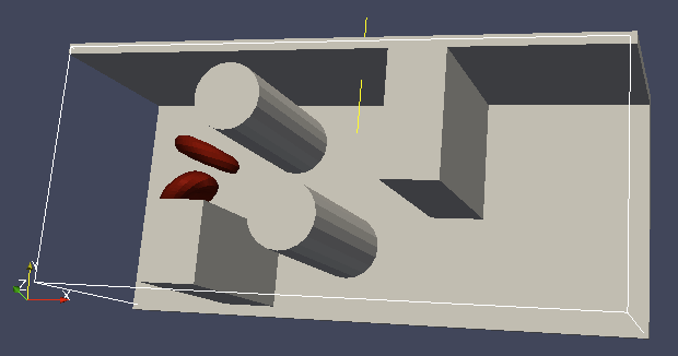
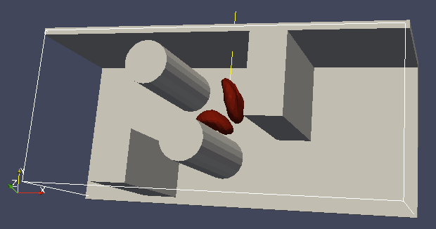
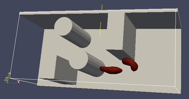
18.5.2.3. Specification of boundaries
To set up the geometry of the channels, we mostly use rhomboids and cylinders, but there are also other shape types available in ESPResSo. Their usage is described elsewhere.

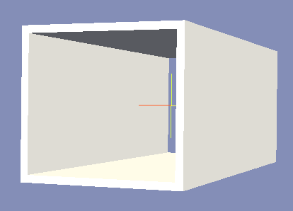
Each wall and obstacle has to be specified separately as a fluid boundary and as a particle constraint. The former enters the simulation as a boundary condition for the fluid, the latter serves for particle-boundary interactions. Sample cylinder and rhomboid can then be defined as follows. First we define the two shapes:
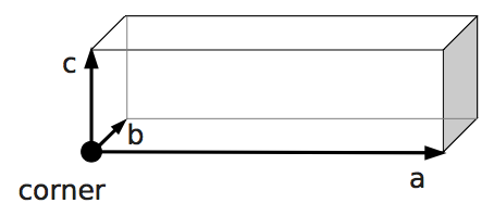
boundary1 = shapes.Rhomboid(corner=[0.0, 0.0, 0.0],
                            a=[boxX, 0.0, 0.0],
                            b=[0.0, boxY, 0.0],
                            c=[0.0, 0.0, 1.0],
                            direction=1)
boundary2 = shapes.Cylinder(center=[11.0, 2.0, 7.0],
                            axis=[0.0, 0.0, 1.0],
                            length=7.0,
                            radius=2.0,
                            direction=1)
The direction=1 determines that the fluid is on the outside. Next
we mark the LB nodes within the shapes as boundaries:
lbf.add_boundary_from_shape(boundary1)
lbf.add_boundary_from_shape(boundary2)
Followed by creating the constraints for cells:
system.constraints.add(shape=boundary1, particle_type=10)
system.constraints.add(shape=boundary2, particle_type=10)
The particle_type=10 will be important for specifying cell-wall
interactions later. And finally, we output the boundaries for
visualisation:
output_vtk_rhomboid(corner=[0.0, 0.0, 0.0],
                    a=[boxX, 0.0, 0.0],
                    b=[0.0, boxY, 0.0],
                    c=[0.0, 0.0, 1.0],
                    out_file="output/sim1/wallBack.vtk")
output_vtk_cylinder(center=[11.0, 2.0, 7.0],
                    axis=[0.0, 0.0, 1.0],
                    length=7.0,
                    radius=2.0,
                    n=20,
                    out_file="output/sim1/obstacle.vtk")
Note that the method for cylinder output also has an argument n.
This specifies number of rectangular faces on the side.
It is a good idea to output and visualize the boundaries and objects just prior to running the actual simulation, to make sure that the geometry is correct and no objects intersect with any boundaries.
18.5.2.4. Specification of interactions
We can define an interaction with the boundaries:
system.non_bonded_inter[0, 10].soft_sphere.set_params(
    soft_a=0.0001, soft_n=1.2, soft_cut=0.1, soft_offset=0.0)
These interactions are also pointwise, e.g. each particle of type 0
(that means all mesh points of cell) will have a repulsive soft-sphere
interaction with all boundaries of type 10 (here all boundaries) once it
gets closer than soft_cut. The parameters soft_a and soft_n
adjust how strong the interaction is and soft_offset is a distance
offset, which will always be zero for our purposes.
18.5.2.5. System integration
And finally, the heart of this script is the integration loop at the end:
for i in range(1, 101):
    system.integrator.run(steps=500)
    cell.output_vtk_pos_folded(filename=f"output/sim1/cell_{i}.vtk")
    print(f"time: {i * time_step}")
print("Simulation completed.")
This simulation runs for 100 cycles. In each cycle, 500 integration
steps are performed and output is saved into files
output/sim1/cell_*.vtk. Note that they differ only by the number
before the .vtk extension (this variable changes due to the for
loop) and this will allow us to animate them in the visualisation
software. str changes the type of i from integer to string, so
that it can be used in the filename. The strings can be joined together
by the + sign. Also, in each pass of the loop, the simulation time is
printed in the terminal window and when the integration is complete, we
should get a message about it.
To sum up, the proper order of setting up individual simulation parts is as follows:
cell types
cells
fluid
fluid boundaries
interactions
If cell types and cells are specified after the fluid, the simulation is slower. Also, interactions can only be defined once the objects and boundaries both exist. Technically, the fluid boundaries can be specified before fluid, but it is really not recommended.
18.5.2.6. Running the simulation
The script can be executed in the terminal with
../pypresso script.py
Here script.py is the name of the script we just went over and
../pypresso should be replaced with the path to your executable.
This command assumes that we are currently in the same directory as the
script. Once the command is executed, messages should appear on the
terminal about the creation of cell type, cell and the integration
steps.
18.5.2.7. Writing out data
In the script, we have used the commands such as
cell.output_vtk_pos_folded(filename=f"output/sim1/cell_{i}.vtk")
to output the information about cell in every pass of the simulation loop. These files can then be used for inspection in ParaView and creation of animations. It is also possible to save a .vtk file for the fluid. And obviously, one can save various types of other data into text or data files for further processing and analysis.
18.5.3. Visualization in ParaView
For visualization we suggest the free software ParaView 5. All .vtk files (boundaries, fluid, objects at all time steps) can be loaded at the same time. The loading is a two step process, because only after pressing the Apply button, are the files actually imported. Using the eye icon to the left of file names, one can turn on and off the individual objects and/or boundaries.
Fluid can be visualized using Filters/Alphabetical/Glyph (or other options from this menu. Please, refer to the ParaView user’s guide for more details).
Note, that ParaView does not automatically reload the data if they have been changed in the input folder, but a useful thing to know is that the created filters can be “recycled”. Once you delete the old data, load the new data and right-click on the existing filters, you can re-attach them to the new data.
It is a good idea to output and visualize the boundaries and objects just prior to running the actual simulation, to make sure that the geometry is correct and no objects intersect with any boundaries. This would cause “particle out of range” error and crash the simulation.
18.5.3.1. File format
ParaView (download at https://www.paraview.org) accepts .vtk files. For our cells we use the following format:
# vtk DataFile Version 3.0
Data
ASCII
DATASET POLYDATA
POINTS 393 float
p0x p0y p0z
p1x p1y p1z
...
p391x p391y p391z
p392x p392y p392z
TRIANGLE_STRIPS num_triang 4*num_triang
3 p1 p2 p3
3 p1 p3 p5
...
3 p390 p391 p392
where the cell has 393 surface nodes (particles). After initial
specification, the list of points is present, with x, y, z coordinates for
each. Then we write the triangulation, since that is how our
surface is specified. We need to know the number of triangles
(num_triang) and the each line/triangle is specified by 4 numbers
(so we are telling ParaView to expect 4 * num_triang numbers in
the following lines. Each line begins with 3 (which stands for a
triangle) and three point IDs that tell us which three points (from
the order above) form this specific triangle.
18.5.3.2. Color coding of scalar data by surface points
It is possible to save (and visualize) data corresponding to individual surface points. These data can be scalar or vector values associated with all surface points. At the end of the .vtk file above, add the following lines:
POINT_DATA 393
SCALARS sample_scalars float 1
LOOKUP_TABLE default
value-at-p0
value-at-p1
...
value-at-p392
This says that data for each of 393 points are coming. Next line says that the data are scalar in this case, one float for each point. To color code the values in the visualization, a default (red-to-blue) table will be used. It is also possible to specify your own lookup table. As an example, we might want to see a force magnitude in each surface node
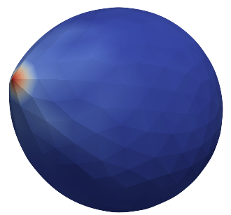
Stretched sphere after some relaxation, showing magnitude of total stretching force in each node.
18.5.3.3. Color coding of scalar data by triangles
It is also possible to save (and visualize) data corresponding to individual triangles
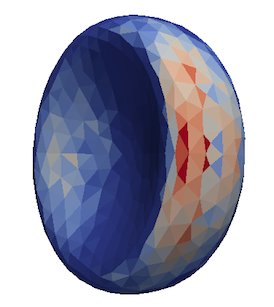
Red blood cell showing which triangles (local surface areas) are under most strain in shear flow.
In such case, the keyword POINT_DATA is changed to CELL_DATA and the number of
triangles is given instead of number of mesh points.
# vtk DataFile Version 3.0
Data
ASCII
DATASET POLYDATA
POINTS 4 float
1 1 1
3 1 1
1 3 1
1 1 3
TRIANGLE_STRIPS 3 12
3 0 1 2
3 0 2 3
3 0 1 3
CELL_DATA 3
SCALARS sample_scalars float 1
LOOKUP_TABLE default
0.0
0.5
1.0
Note - it is also possible to save (and visualize) data corresponding to edges.
18.5.3.4. Multiple scalar data in one .vtk file
If one wants to switch between several types of scalar values corresponding to mesh nodes, these are specifies consecutively in the .vtk file, as follows. Their names (scalars1 and scalars2 in the following example) appear in a drop-down menu in ParaView.
POINT_DATA 393
SCALARS scalars1 float 1
LOOKUP_TABLE default
value1-at-p0
value1-at-p1
...
value1-at-p392
SCALARS scalars2 float 1
LOOKUP_TABLE default
value2-at-p0
value2-at-p1
...
value2-at-p392
18.5.3.5. Vector data for objects .vtk file
POINT_DATA 393
VECTORS vector_field float
v1-at-p0 v2-at-p0 v3-at-p0
v1-at-p1 v2-at-p1 v3-at-p1
...
v1-at-p391 v2-at-p391 v3-at-p392
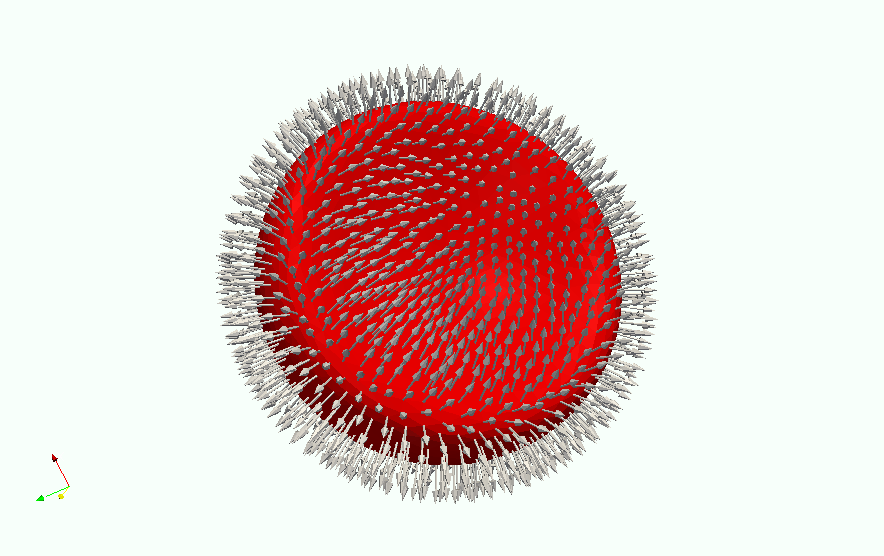
Example of vector data stored in points of the object
18.5.3.6. Automatic loading
paraview --script=loading-script.py and all the steps for creating
that scenario will be executed and you end up with the velocity field
visualized.18.5.4. Available Object-in-fluid (OIF) classes
keywords, parameter values, vectors18.5.4.1. class OifCellType
For those familiar with earlier version of object-in-fluid framework, this class corresponds to the oif_emplate in tcl. It contains a “recipe” for creating cells of the same type. These cells can then be placed at different locations with different orientation, but their elasticity and size is determined by the CellType. There are no actual particles created at this stage. Also, while the interactions are defined, no bonds are created here.
OifCellType.print_info()
OifCellType.mesh.output_mesh_triangles(filename)
nodesfile=nodes.dat - input file. Each line contains three
real numbers. These are the x, y, z coordinates of individual
surface mesh nodes of the objects centered at [0,0,0] and normalized
so that the “radius” of the object is 1.trianglesfile=triangles.dat - input file. Each line contains
three integers. These are the ID numbers of the mesh nodes as they
appear in nodes.dat. Note that the first node has ID 0.system=system Particles of cells created using this
template will be added to this system. Note that there can be only one
system per simulation.ks=value - elastic modulus for stretching forces.kslin= value - elastic modulus for linear stretching forces.kb= value - elastic modulus for bending forces.kal= value - elastic modulus for local area forces.ks, kb and kal set elastic parameters for
local interactions: ks for edge stiffness, kb for angle
preservation stiffness and kal for triangle area preservation
stiffness. Currently, the stiffness is implemented to be uniform over
the whole object, but with some tweaking, it is possible to have
non-uniform local interactions.ks) and linear stretching
(kslin) - these two options cannot be used simultaneously:kvisc=value - elastic modulus for viscosity of the membrane.
Viscosity slows down the reaction of the membrane.kag=value - elastic modulus for global area forceskv=value - elastic modulus for volume forcesresize=(x, y, z) - coefficients, by which the coordinates
stored in nodesfile will be stretched in the x, y, z
direction. The default value is (1.0, 1.0, 1.0).mirror=(x, y, z) - whether the respective coordinates should
be flipped around 0. Arguments x, y, z must be either 0 or 1.
The reflection of only one coordinate is allowed so at most one
argument is set to 1, others are 0. For example mirror=(0, 1, 0)
results in flipping the coordinates (x, y, z) to (x, -y, z). The
default value is (0, 0, 0).normal - by default set to False, however without this
option enabled, the membrane collision (and thus cell-cell
interactions) will not work.check_orientation - by default set to True. This options
performs a check, whether the supplied trianglesfile contains
triangles with correct orientation. If not, it corrects the
orientation and created cells with corrected triangles. It is useful
for new or unknown meshes, but not necessary for meshes that have
already been tried out. Since it can take a few minutes for larger
meshes (with thousands of nodes), it can be set to False. In
that case, the check is skipped when creating the CellType and a
warning is displayed.CellType.mesh.OutputMeshTriangles(filename), so that the
check does not have to be used repeatedly.CellType.mesh.output_mesh_triangles(filename) - this is
useful after checking orientation, if any of the triangles where
corrected. This method saves the current triangles into a file that
can be used as input in the next simulations.CellType.print_info() - prints the information about the template.18.5.4.2. class OifCell
OifCell.set_origin([x, y, z])
OifCell.get_origin()
OifCell.get_origin_folded()
OifCell.get_approx_origin()
OifCell.get_velocity()
OifCell.set_velocity([x, y, z])
OifCell.pos_bounds()
OifCell.surface()
OifCell.volume()
OifCell.diameter()
OifCell.get_n_nodes()
OifCell.set_force([x, y, z])
OifCell.kill_motion()
OifCell.unkill_motion()
OifCell.output_vtk_pos(filename.vtk)
OifCell.output_vtk_pos_folded(filename.vtk)
OifCell.append_point_data_to_vtk(filename.vtk, dataname, data, firstAppend)
OifCell.output_raw_data(filename, rawdata)
OifCell.output_mesh_points(filename)
OifCell.set_mesh_points(filename)
OifCell.elastic_forces(elasticforces, fmetric, vtkfile, rawdatafile)
OifCell.print_info()
cell_type - object will be created using nodes, triangle
incidences, elasticity parameters and initial stretching saved in this
cellType.part_type=type - must start at 0 for the first cell and
increase consecutively for different cells. Volume calculation of
individual objects and interactions between objects are set up using
these types.origin=(x, y, z) - center of the object will be at this
point.rotate=(x, y, z) - angles in radians, by which the object
will be rotated about the x, y, z axis. Default value is (0.0,
0.0, 0.0). Value (\(\pi/2, 0.0, 0.0\)) means that the object will
be rotated by \(\pi/2\) radians clockwise around the x
axis when looking in the positive direction of the axis.mass=m - mass of one particle. Default value is 1.0.OifCell.set_origin(o) - moves the object such that the origin
has coordinates o=(x, y, z).OifCell.get_origin() - outputs the location of the center of the
object.OifCell.get_origin_folded() - outputs the location of the center of
the object. For periodical movements the coordinates are folded
(always within the computational box).OifCell.get_approx_origin() - outputs the approximate location of
the center of the object. It is computed as average of 6 mesh points
that have extremal x, y and z coordinates at the time
of object loading.OifCell.get_velocity() - outputs the average velocity of the
object. Runs over all mesh points and outputs their average velocity.OifCell.set_velocity(v) - sets the velocities of all mesh
points to v=(\(v_x\), \(v_y\), \(v_z\)).OifCell.pos_bounds() - computes six extremal coordinates of the
object. More precisely, runs through the all mesh points and returns
the minimal and maximal \(x\)-coordinate, \(y\)-coordinate and
\(z\)-coordinate in the order (\(x_{max}\), \(x_{min}\),
\(y_{max}\), \(y_{min}\), \(z_{max}\), \(z_{min}\)).OifCell.surface() - outputs the surface of the object.OifCell.volume() - outputs the volume of the object.OifCell.diameter() - outputs the largest diameter of the object.OifCell.get_n_nodes() - returns the number of mesh nodes.OifCell.set_force(f) - sets the external force vector
f=(\(f_x\), \(f_y\), \(f_z\)) to all mesh nodes of
the object. Setting is done using command p.set_force(f).
Note, that this command sets the external force in each integration
step. So if you want to use the external force only in one iteration,
you need to set zero external force in the following integration step.OifCell.kill_motion() - stops all the particles in the object
(analogue to the command p.kill_motion()).OifCell.unkill_motion() - enables the movement of all the particles
in the object (analogue to the command p.unkill_motion()).OifCell.output_vtk_pos(filename.vtk) - outputs the mesh of the
object to the desired filename.vtk. ParaView can directly visualize
this file.OifCell.output_vtk_pos_folded(filename.vtk) - outputs the mesh of
the object to the desired filename.vtk. ParaView can directly
visualize this file. For periodical movements the coordinates are
folded (always within the computational box).OifCell.append_point_data_to_vtk(filename.vtk, dataname,
data, firstAppend) - outputs the specified scalar data to an
existing filename.vtk. This is useful for ParaView
visualisation of local velocity magnitudes, magnitudes of forces, etc.
in the meshnodes and can be shown in ParaView by selecting the
dataname in the Properties toolbar. It is possible to
consecutively write multiple datasets into one filename.vtk.
For the first one, the firstAppend parameter is set to
True, for the following datasets, it needs to be set to
False. This is to ensure the proper structure of the output
file.OifCell.output_raw_data(filename, rawdata) - outputs the
vector rawdata about the object into the filename.OifCell.output_mesh_points(filename) - outputs the positions of
the mesh nodes to filename. In fact, this command creates a new
nodes.dat file that can be used by the method
OifCell.set_mesh_points(nodes.dat). The center of the object is
located at point (0.0, 0.0, 0.0). This command is aimed to store the
deformed shape in order to be loaded later.OifCell.set_mesh_points(filename) - deforms the object in such a
way that its origin stays unchanged, however the relative positions of
the mesh points are taken from file filename. The filename should
contain the coordinates of the mesh points with the origin location at
(0.0, 0.0, 0.0). The procedure also checks whether number of lines in
the filename is the same as the corresponding value from
OifCell.get_n_nodes().OifCell.elastic_forces(elasticforces, fmetric, vtkfile,
rawdatafile) - this method can be used in two different ways. One is
to compute the elastic forces locally for each mesh node and the other
is to compute the f-metric, which is an approximation of elastic
energy.OifCell.print_info() - prints the information about the elastic
object.18.5.4.3. Short utility procedures
get_n_triangle(a, b, c) - returns the normal n
to the triangle given by points (a, b, c).norm(v) - returns the norm of the vector v.distance(a, b) - returns the distance between
points a and b.area_triangle(a, b, c) - returns the area of the
given triangle (a, b, c).angle_btw_triangles(\(\mathbf{p}_1\), \(\mathbf{p}_2\),
\(\mathbf{p}_3\), \(\mathbf{p}_4\) - returns the angle
\(\phi\) between two triangles: (\(\mathbf{p}_1\),
\(\mathbf{p}_2\), \(\mathbf{p}_3\)) and (\(\mathbf{p}_3\),
\(\mathbf{p}_2\), \(\mathbf{p}_4\)) that have a common edge
(\(\mathbf{p}_2\), \(\mathbf{p}_3\)).discard_epsilon(x) - needed for rotation; discards very
small numbers x.oif_neo_hookean_nonlin(\(\lambda\)) - nonlinearity for neo-Hookean stretchingcalc_stretching_force(\(k_s,\ \mathbf{p}_A,\ \mathbf{p}_B\), dist0, dist)
- computes the nonlinear stretching force with given \(k_s\) for
points \(\mathbf{p}_A\) and \(\mathbf{p}_B\) given by their
coordinates, whose initial distance was dist0 and current distance
is dist.calc_linear_stretching_force(\(k_s,\ \mathbf{p}_A,\ \mathbf{p}_B\), dist0, dist)
- computes the linear stretching force with given \(k_s\) for
points \(\mathbf{p}_A\) and \(\mathbf{p}_B\) given by their
coordinates, whose initial distance was dist0 and current distance
is dist.calc_bending_force(\(k_b,\ \mathbf{p}_A,\ \mathbf{p}_B,\ \mathbf{p}_C,\ \mathbf{p}_D,\ \phi_0,\ \phi\))
- computes the bending force with given \(k_b\) for points
\(\mathbf{p}_A\), \(\mathbf{p}_B\), \(\mathbf{p}_C\) and
\(\mathbf{p}_D\) (\(\triangle_1\)=BAC;
\(\triangle_2\)=BCD) given by their coordinates; the initial
angle for these two triangles was \(\phi_0\), the current angle is
\(\phi\).calc_local_area_force(\(k_{al},\ \mathbf{p}_A,\ \mathbf{p}_B,\ \mathbf{p}_C,\ A_0,\ A\))
- computes the local area force with given \(k_{al}\) for points
\(\mathbf{p}_A\), \(\mathbf{p}_B\) and \(\mathbf{p}_C\)
given by their coordinates; the initial area of triangle ABC was
\(A_0\), the current area is \(A\).calc_global_area_force(\(k_{ag},\ \mathbf{p}_A,\ \mathbf{p}_B,\ \mathbf{p}_C,\ A_{g0},\ A_g\))
- computes the global area force with given \(k_{ag}\) for points
\(\mathbf{p}_A\), \(\mathbf{p}_B\) and \(\mathbf{p}_C\)
given by their coordinates; the initial surface area of the object was
\(A_{g0}\), the current surface area of the object is \(A_g\).calc_volume_force(\(k_v,\ \mathbf{p}_A,\ \mathbf{p}_B,\ \mathbf{p}_C,\ V_0,\ V\))
- computes the volume force with given \(k_v\) for points
\(\mathbf{p}_A\), \(\mathbf{p}_B\) and \(\mathbf{p}_C\)
given by their coordinates; the initial volume of the object was
\(V_0\), the current volume of the object is \(V\).output_vtk_rhomboid(corner, a, b, c, outFile.vtk)
- outputs rhomboid boundary for later visualisation in ParaView.output_vtk_cylinder(center, normal, L, r, n, outFile.vtk)
- outputs cylinder boundary for later visualisation in ParaView.output_vtk_lines(lines, outFile.vtk) - outputs a set of
line segments for later visualisation in ParaView.18.5.4.4. Description of helper classes
Awareness of these classes is not necessary for a user of OIF module, but is essential for developers who wish to modify it because it shows how the object data are stored.
classes FixedPoint and PartPoint
Class PartPoint represents a particle. These particles are then used as building blocks for edges, angles, triangles and ultimately the whole object mesh. Since we use a two-step process to create the objects, it is necessary to distinguish between a FixedPoint and PartPoint. FixedPoint is a point used by template and does not correspond to particle. The FixedPoints of one OifCellType form a mesh that is centered around origin. Only after it is stretched and shifted to the object origin are the PartPoints of the given object created.
classes Edge, Angle, Triangle, ThreeNeighbors
These classes represent the building blocks of a mesh. They are used to compute the elastic interactions: Edge is for stretching, Angle for bending, Triangle for local and global area and volume and ThreeNeigbors for calculation of outward normal vector needed for cell-cell interaction.
class Mesh
This class holds all the information about the geometry of the object, including nodes, edges, angles, triangles and neighboring points. The mesh of OifCellType is copied every time a new object (i.e. OifCell) of this type is created. This saves computational time, since the data for elastic interactions of the given object do not need to be recalculated every time.
18.6. Particle polarizability with thermalized cold Drude oscillators
Note
Requires features THOLE, P3M, THERMOSTAT_PER_PARTICLE.
Note
Drude is only available for the P3M electrostatics solver and the Langevin thermostat.
Thermalized cold Drude oscillators can be used to simulate polarizable particles. The basic idea is to add a ‘charge-on-a-spring’ (Drude charge) to a particle (Drude core) that mimics an electron cloud which can be elongated to create a dynamically inducible dipole. The energetic minimum of the Drude charge can be obtained self-consistently, which requires several iterations of the system’s electrostatics and is usually considered computationally expensive. However, with thermalized cold Drude oscillators, the distance between Drude charge and core is coupled to a thermostat so that it fluctuates around the SCF solution. This thermostat is kept at a low temperature compared to the global temperature to minimize the heat flow into the system. A second thermostat is applied on the centre of mass of the Drude charge + core system to maintain the global temperature. The downside of this approach is that usually a smaller time step has to be used to resolve the high frequency oscillations of the spring to get a stable system.
In ESPResSo, the basic ingredients to simulate such a system are split into three bonds:
A Harmonic bond to account for the spring.
A Thermalized distance bond with a cold thermostat on the Drude-Core distance.
A Subtract P3M short-range bond to cancel the electrostatic interaction between Drude and core particles.
The system-wide thermostat has to be applied to the centre of mass and not to
the core particle directly. Therefore, the particles have to be excluded from
global thermostatting. With THERMOSTAT_PER_PARTICLE enabled, we set the
friction coefficient of the Drude complex to zero, which allows
to still use a global Langevin thermostat for non-polarizable particles.
As the Drude charge should not alter the charge or mass of the Drude complex, both properties have to be subtracted from the core when adding the Drude particle. In the following convention, we assume that the Drude charge is always negative. It is calculated via the spring constant \(k\) and polarizability \(\alpha\) (in units of inverse volume) with \(q_d = -\sqrt{k \cdot \alpha}\).
The following helper method takes into account all the preceding considerations and can be used to conveniently add a Drude particle to a given core particle. It returns an espressomd.particle_data.ParticleHandle to the created Drude particle. Note that as the function also adds the first two bonds between Drude and core, these bonds have to be already available.:
import espressomd.drude_helpers
dh = espressomd.drude_helpers.DrudeHelpers()
drude_part = dh.add_drude_particle_to_core(<system>, <harmonic_bond>,
    <thermalized_bond>, <core particle>, <type drude>, <alpha>,
    <mass drude>, <coulomb_prefactor>, <thole damping>, <verbose>)
- The arguments of the helper function are:
<system>: Theespressomd.System().<harmonic_bond>: The harmonic bond of the charge-on-a-spring. This is added between core and newly generated Drude particle<thermalized_bond>: The thermalized distance bond for the cold and hot thermostats.<core particle>: The core particle on which the Drude particle is added.<type drude>: The user-defined type of the Drude particle. Each Drude particle of each complex should have an individual type (e.g. in an ionic system with Anions (type 0) and Cations (type 1), two new, individual Drude types have to be assigned).<alpha>: The polarizability volume.<coulomb_prefactor>: The Coulomb prefactor of the system. Used to calculate the Drude charge from the polarizability and the spring constant of the Drude bond.<thole damping>: (optional) An individual Thole damping parameter for the core-Drude pair. Only relevant if Thole damping is used (defaults to 2.6).<verbose>: (bool, optional) Prints out information about the added Drude particles (default: False)
What is still missing is the short-range exclusion bond between all Drude-core pairs. One bond type of this kind is needed per Drude type. The above helper function also tracks particle types, ids and charges of Drude and core particles, so a simple call of another helper function:
dh.setup_and_add_drude_exclusion_bonds(system)
will use this data to create a Subtract P3M short-range bond per Drude type
and set it up it between all Drude and core particles collected in calls of
add_drude_particle_to_core().
18.6.1. Canceling intramolecular electrostatics
Note that for polarizable molecules (i.e. connected particles, coarse grained models etc.) with partial charges on the molecule sites, the Drude charges will have electrostatic interaction with other cores of the molecule. Often, this is unwanted, as it might be already part of the force-field (via. partial charges or parametrization of the covalent bonds). Without any further measures, the elongation of the Drude particles will be greatly affected be the close-by partial charges of the molecule. To prevent this, one has to cancel the interaction of the Drude charge with the partial charges of the cores within the molecule. This can be done with special bonds that subtracts the P3M short-range interaction of the charge portion \(q_d q_{partial}\). This ensures that only the dipolar interaction inside the molecule remains. It should be considered that the error of this approximation increases with the share of the long-range part of the electrostatic interaction. Two helper methods assist with setting up this exclusion. If used, they have to be called after all Drude particles are added to the system:
espressomd.drude_helpers.setup_intramol_exclusion_bonds(<system>, <molecule drude types>,
    <molecule core types>, <molecule core partial charges>, <verbose>)
This function creates the required number of bonds which are later added to the particles. It has to be called only once. In a molecule with \(N\) polarizable sites, \(N \cdot (N-1)\) bond types are needed to cover all the combinations. Parameters are:
<system>: Theespressomd.System().<molecule drude types>: List of the Drude types within the molecule.<molecule core types>: List of the core types within the molecule that have partial charges.<molecule core partial charges>: List of the partial charges on the cores.<verbose>: (bool, optional) Prints out information about the created bonds (default: False)
After setting up the bonds, one has to add them to each molecule with the following method:
espressomd.drude_helpers.add_intramol_exclusion_bonds(<system>, <drude ids>, <core ids>, <verbose>)
This method has to be called for all molecules and needs the following parameters:
<system>: Theespressomd.System().<drude ids>: The ids of the Drude particles within one molecule.<core ids>: The ids of the core particles within one molecule.<verbose>: (bool, optional) Prints out information about the added bonds (default:False)
Internally, this is done with the bond described in Subtract P3M short-range bond, that simply adds the p3m shortrange pair-force of scale \(- q_{\textrm{d}} q_{\textrm{partial}}\) the to bonded particles.
See also
Often used in conjunction with Drude oscillators is the Thole correction to damp dipole-dipole interactions on short distances. It is available in ESPResSo as a non-bonded interaction.